ArviZ migration guide#
We have been working on refactoring ArviZ to allow more flexibility and extensibility of its elements while keeping as much as possible a friendly user-interface that gives sensible results with little to no arguments.
One important change is enhanced modularity. Everything will still be available through a common namespace arviz,
but ArviZ will now be composed of 3 smaller libraries:
arviz-base data related functionality, including converters from different PPLs.
arviz-stats for statistical functions and diagnostics.
arviz-plots for visual checks built on top of arviz-stats and arviz-base.
Each library has a minimal set of dependencies, with a lot of functionality built on top of optional dependencies. This keeps ArviZ smaller and easier to install as you can install only the components you really need. The main examples are:
arviz-basehas no I/O library as a dependency, but you can usenetcdf4,h5netcdforzarrto read and write your data, allowing you to install only the one you need.arviz-plotshas no plotting library as a dependency, but it can generate plots withmatplotlib,bokehorplotlyif they are installed.
import arviz as az
Check all 3 libraries have been exposed correctly:
print(az.info)
Status information for ArviZ 1.0.0rc0
arviz_base 0.9.0.dev0 available, exposing its functions as part of the `arviz` namespace
arviz_stats 0.9.0.dev available, exposing its functions as part of the `arviz` namespace
arviz_plots 0.9.0.dev0 available, exposing its functions as part of the `arviz` namespace
arviz-base#
Credible intervals and rcParams#
Some global configuration settings have changed. For example, the default credible interval probability (ci_prob) has been updated from 0.94 to 0.89. Using 0.89 produces intervals with lower variability, leading to more stable summaries. At the same time, keeping a non-standard value (rather than 0.90 or 0.95) serves as a friendly reminder that the choice of interval can depend on the problem at hand.
In addition, a new setting ci_kind has been introduced, which defaults to “eti” (equal-tailed interval). This controls the method used to compute credible intervals. The alternative is “hdi” (highest density interval), which was previously the default.
Defaults set via rcParams are not fixed rules, they’re meant to be adjusted to fit the needs of your analysis. rcParams offers a convenient way to establish global defaults for your workflow, while most functions that compute credible intervals also provide ci_prob and ci_kind arguments to override these settings locally.
You can check all default settings with:
az.rcParams
RcParams({'data.http_protocol': 'https',
'data.index_origin': 0,
'data.sample_dims': ('chain', 'draw'),
'data.save_warmup': False,
'plot.backend': 'matplotlib',
'plot.density_kind': 'kde',
'plot.max_subplots': 40,
'stats.ci_kind': 'eti',
'stats.ci_prob': 0.89,
'stats.envelope_prob': 0.99,
'stats.ic_compare_method': 'stacking',
'stats.ic_pointwise': True,
'stats.ic_scale': 'log',
'stats.module': 'base',
'stats.point_estimate': 'mean',
'stats.round_to': '2g'})
DataTree#
One of the main differences is that the arviz.InferenceData object doesn’t exist anymore.
arviz-base uses xarray.DataTree instead. This is a new data structure in xarray,
so it might still have some rough edges, but it is much more flexible and powerful.
To give some examples, I/O will now be more flexible, and any format supported by
xarray is automatically available to you, no need to add wrappers on top of them within ArviZ.
It is also possible to have arbitrary nesting of variables within groups and subgroups.
Important
Not all the functionality on xarray.DataTree will be compatible with ArviZ as it would be too much
work for us to cover and maintain. If there are things you have always wanted to do but
were not possible with InferenceData and are now possible with DataTree please try
them out, give feedback on them and on desired behaviour for things that still don’t work.
After a couple releases the “ArviZverse” will stabilize much more, and it might not be
possible to add support for that anymore.
What about my existing netcdf/zarr files?#
They are still valid. There have been no changes on this end and we don’t plan to make any. The underlying functions handling I/O operations have changed, but the effect on your workflows should be minimal; the arguments continue to be mostly the same, and only some duplicated aliases have been removed:
Function in legacy ArviZ |
New equivalent in xarray |
|---|---|
arviz.from_netcdf |
|
arviz.from_zarr |
|
arviz.to_netcdf |
- |
arviz.to_zarr |
- |
arviz.InferenceData.from_netcdf |
- |
arviz.InferenceData.from_zarr |
- |
arviz.InferenceData.to_netcdf |
|
arviz.InferenceData.to_zarr |
from_zarris afunctools.partialwrapper ofopen_datatreewithengine="zarr"already setfrom_netcdfis exactlyopen_datatreeso you can use theenginekeyword to choose explicitly betweennetcdf4,h5netcdfor leave it to xarray’s default behaviour andnetcdf_engine_ordersetting.
Here is an example where we read a file that was saved from an InferenceData object using idata.to_netcdf("example.nc").
dt = az.from_netcdf("example.nc")
dt
<xarray.DataTree>
Group: /
├── Group: /posterior
│ Dimensions: (chain: 4, draw: 500, school: 8)
│ Coordinates: (3)
│ Data variables:
│ mu (chain, draw) float64 16kB ...
│ theta (chain, draw, school) float64 128kB ...
│ tau (chain, draw) float64 16kB ...
│ Attributes: (6)
├── Group: /posterior_predictive
│ Dimensions: (chain: 4, draw: 500, school: 8)
│ Coordinates: (3)
│ Data variables:
│ obs (chain, draw, school) float64 128kB ...
│ Attributes: (4)
├── Group: /log_likelihood
│ Dimensions: (chain: 4, draw: 500, school: 8)
│ Coordinates: (3)
│ Data variables:
│ obs (chain, draw, school) float64 128kB ...
│ Attributes: (4)
...
├── Group: /prior_predictive
│ Dimensions: (chain: 1, draw: 500, school: 8)
│ Coordinates: (3)
│ Data variables:
│ obs (chain, draw, school) float64 32kB ...
│ Attributes: (4)
├── Group: /observed_data
│ Dimensions: (school: 8)
│ Coordinates: (1)
│ Data variables:
│ obs (school) float64 64B ...
│ Attributes: (4)
└── Group: /constant_data
Dimensions: (school: 8)
Coordinates: (1)
Data variables:
sigma (school) float64 64B ...
Attributes: (4)Other key differences#
Because DataTree is an xarray object intended for a broader audience; its methods differ from those of InferenceData.
This section goes over the main differences to help migrate code that used InferenceData to now use DataTree.
DataTree supports an arbitrary level of nesting (as opposed to the exactly 1 level of nesting in
InferenceData). To stay consistent, accessing a group always returns a DataTree,
even when the group is a leaf (that is, it contains no further subgroups).
This means that dt["posterior"] will now return a DataTree.
In many cases this is irrelevant, but there will be some cases where you’ll want the
group as a Dataset instead. You can achieve this with either dt["posterior"].dataset if you only need a view,
or dt["posterior"].to_dataset() to get a new copy if you want a mutable Dataset.
There are no changes at the variable/DataArray level. Thus, dt["posterior"]["theta"] is still
a DataArray, accessing its variables is one of the cases where having either DataTree
or Dataset is irrelevant.
InferenceData.extend#
Another extremely common method of InferenceData was .extend. In this case, the same behaviour can be replicated with xarray.DataTree.update() which behaves like the method of the same name in dict objects. These are the two equivalences:
idata.extend(idata_new)
idata_new.update(idata)
# or
idata.extend(idata_new, how="right")
idata.update(idata_new)
The default behaviour in .extend was to do a “left-like merge”. That is, if both idata and idata_new have an observed_data group, .extend preserved the one in idata
and ignored that group in idata_new. Using .update with the switched order we get the same behaviour as any repeated groups in idata will overwrite the ones in idata_new.
For cases that explicitly set how="right" then .update should use the same order as .extend did.
InferenceData.map#
The .map method is very similar to xarray.DataTree.map_over_datasets(). The main difference is the lack of groups, filter_groups and inplace arguments.
In order to achieve this we need to combine .map_over_datasets with either filter() or match().
For example, applying a function to only the posterior_predictive and prior_predictive group which used to be
idata.map(lambda ds: ds + 3, groups="_predictive", filter_groups="like")
can now be partially achieved with (we’ll see the the full equivalence later on):
dt.match("*_predictive").map_over_datasets(lambda ds: ds + 3)
<xarray.DataTree>
Group: /
├── Group: /posterior_predictive
│ Dimensions: (chain: 4, draw: 500, school: 8)
│ Coordinates: (3)
│ Data variables:
│ obs (chain, draw, school) float64 128kB 41.88 -11.98 ... 30.05 23.99
│ Attributes: (4)
└── Group: /prior_predictive
Dimensions: (chain: 1, draw: 500, school: 8)
Coordinates: (3)
Data variables:
obs (chain, draw, school) float64 32kB 25.03 29.95 ... 61.23 42.78
Attributes: (4)If we instead want to apply it also to the observed_data group, it is no longer as easy to use glob-like patterns. We can use filter instead to check against a list, which is similar to using a list/tuple as the groups argument:
dt.filter(
lambda node: node.name in ("posterior_predictive", "prior_predictive", "observed_data")
).map_over_datasets(lambda ds: ds + 3)
<xarray.DataTree>
Group: /
├── Group: /posterior_predictive
│ Dimensions: (chain: 4, draw: 500, school: 8)
│ Coordinates: (3)
│ Data variables:
│ obs (chain, draw, school) float64 128kB 41.88 -11.98 ... 30.05 23.99
│ Attributes: (4)
├── Group: /prior_predictive
│ Dimensions: (chain: 1, draw: 500, school: 8)
│ Coordinates: (3)
│ Data variables:
│ obs (chain, draw, school) float64 32kB 25.03 29.95 ... 61.23 42.78
│ Attributes: (4)
└── Group: /observed_data
Dimensions: (school: 8)
Coordinates: (1)
Data variables:
obs (school) float64 64B 31.0 11.0 0.0 10.0 2.0 4.0 21.0 15.0
Attributes: (4)In both cases we have created a whole new DataTree with only the groups we have filtered and applied functions to.
This is often not what we want when working with DataTree objects that follow the InferenceData schema.
The default behaviour of .map (or any InferenceData method that took a groups argument) was to act on the selected groups,
leave the rest untouched and return all groups in the output. We can achieve this and fully reproduce .map using also .update.
shifted_dt = dt.copy()
shifted_dt.update(dt.match("*_predictive").map_over_datasets(lambda ds: ds + 3))
shifted_dt
<xarray.DataTree>
Group: /
├── Group: /posterior
│ Dimensions: (chain: 4, draw: 500, school: 8)
│ Coordinates: (3)
│ Data variables:
│ mu (chain, draw) float64 16kB ...
│ theta (chain, draw, school) float64 128kB ...
│ tau (chain, draw) float64 16kB ...
│ Attributes: (6)
├── Group: /posterior_predictive
│ Dimensions: (chain: 4, draw: 500, school: 8)
│ Coordinates: (3)
│ Data variables:
│ obs (chain, draw, school) float64 128kB 41.88 -11.98 ... 30.05 23.99
│ Attributes: (4)
├── Group: /log_likelihood
│ Dimensions: (chain: 4, draw: 500, school: 8)
│ Coordinates: (3)
│ Data variables:
│ obs (chain, draw, school) float64 128kB ...
│ Attributes: (4)
...
├── Group: /prior_predictive
│ Dimensions: (chain: 1, draw: 500, school: 8)
│ Coordinates: (3)
│ Data variables:
│ obs (chain, draw, school) float64 32kB 25.03 29.95 ... 61.23 42.78
│ Attributes: (4)
├── Group: /observed_data
│ Dimensions: (school: 8)
│ Coordinates: (1)
│ Data variables:
│ obs (school) float64 64B ...
│ Attributes: (4)
└── Group: /constant_data
Dimensions: (school: 8)
Coordinates: (1)
Data variables:
sigma (school) float64 64B ...
Attributes: (4)In order to replicate the inplace=True behaviour you can skip the .copy part.
Tip
Other methods like .sel are already present in DataTree and generally serve as drop-in replacements.
But there is also the difference of groups, filter_groups and inplace.
The patterns shown here for .map_over_datasets can be used with any method we want to apply to a subset of groups.
InferenceData.groups#
DataTree continues to have a .groups attribute, but due to its support for arbitrary nesting, the groups are returned as unix directory paths:
dt.groups
('/',
'/posterior',
'/posterior_predictive',
'/log_likelihood',
'/sample_stats',
'/prior',
'/prior_predictive',
'/observed_data',
'/constant_data')
To check against .groups we’d need do something like f"/{group}" in dt.groups which might be annoying (but necessary if we want to test for groups nested more than one level).
In our case, we usually restrict ourselves to a single level of nesting in which case it can be more convenient to check things against .children
"posterior" in dt.children
True
The .children attribute is a dict-like view of the nodes at the immediately lower level in the hierarchy. When checking for presence of groups this doesn’t matter as we have seen, but to get a list of groups like the old InferenceData.groups you need to convert it explicitly:
list(dt.children)
['posterior',
'posterior_predictive',
'log_likelihood',
'sample_stats',
'prior',
'prior_predictive',
'observed_data',
'constant_data']
Enhanced converter flexibility#
Were you constantly needing to add an extra axis to your data because it didn’t have any chain dimension? No more!
import numpy as np
rng = np.random.default_rng()
data = rng.normal(size=1000)
# arviz_legacy.from_dict({"posterior": {"mu": data}}) would fail
# unless you did data[None, :] to add the chain dimension
az.rcParams["data.sample_dims"] = "sample"
dt = az.from_dict({"posterior": {"mu": data}})
dt
<xarray.DataTree>
Group: /
└── Group: /posterior
Dimensions: (sample: 1000)
Coordinates: (1)
Data variables:
mu (sample) float64 8kB 0.4879 -0.4405 0.4089 ... 1.147 -0.3469 0.4506
Attributes: (4)# arviz-stats and arviz-plots also take it into account
az.plot_dist(dt);
Note
It is also possible to modify sample_dims through arguments to the different functions.
New data wrangling features#
We have also added multiple functions to help with common data wrangling tasks,
mostly from and to xarray.Dataset. For example, you can convert a dataset
to a wide format dataframe with unique combinations of sample_dims as its rows,
with dataset_to_dataframe():
# back to default behaviour
az.rcParams["data.sample_dims"] = ["chain", "draw"]
dt = az.load_arviz_data("centered_eight")
az.dataset_to_dataframe(dt.posterior.dataset)
| mu | theta[Choate] | theta[Deerfield] | theta[Phillips Andover] | theta[Phillips Exeter] | theta[Hotchkiss] | theta[Lawrenceville] | theta[St. Paul's] | theta[Mt. Hermon] | tau | |
|---|---|---|---|---|---|---|---|---|---|---|
| (0, 0) | 1.715723 | 2.317391 | 1.450174 | 2.085550 | 2.227076 | 3.071507 | 2.712972 | 3.083764 | 1.460448 | 0.877494 |
| (0, 1) | 1.903481 | 0.889170 | 0.742949 | 3.125869 | 2.779524 | 2.834705 | 1.558939 | 2.487503 | 1.984379 | 0.802714 |
| (0, 2) | 1.903481 | 0.889170 | 0.742949 | 3.125869 | 2.779524 | 2.834705 | 1.558939 | 2.487503 | 1.984379 | 0.802714 |
| (0, 3) | 1.903481 | 0.889170 | 0.742949 | 3.125869 | 2.779524 | 2.834705 | 1.558939 | 2.487503 | 1.984379 | 0.802714 |
| (0, 4) | 2.017497 | 1.109120 | 0.818893 | 2.750620 | 1.928670 | 1.983162 | 1.029620 | 3.662744 | 2.167574 | 0.767934 |
| ... | ... | ... | ... | ... | ... | ... | ... | ... | ... | ... |
| (3, 495) | 7.750625 | 11.477589 | 5.578327 | 9.321531 | 5.812095 | 5.437099 | 3.096142 | 9.731409 | 7.948321 | 3.020477 |
| (3, 496) | 6.922368 | 2.710763 | 8.646136 | 3.807844 | 7.543669 | 6.788881 | 6.595036 | 4.003042 | 5.275016 | 2.704639 |
| (3, 497) | 5.408836 | 11.406390 | 4.446937 | 9.210775 | 6.331074 | 4.150778 | 4.812302 | 9.693257 | 4.914656 | 2.236486 |
| (3, 498) | 7.721440 | 7.086139 | 12.311889 | 6.584301 | 10.286093 | 10.050167 | 11.859938 | 7.952268 | 9.754468 | 2.989656 |
| (3, 499) | 10.237157 | 10.464390 | 13.714306 | 10.261666 | 15.180098 | 10.916030 | 15.070900 | 14.923210 | 14.023129 | 3.051559 |
2000 rows × 10 columns
Note it is also aware of ArviZ naming conventions in addition to using
the sample_dims rcParam. It can be further customized through a labeller argument.
Tip
If you want to convert to a long format dataframe, you should use
xarray.Dataset.to_dataframe() instead.
arviz-stats#
Stats and diagnostics related functionality have also had some changes, and it should also be noted that out of the 3 new modular libraries it is currently the one lagging behind a bit more. At the same time, it does already have several new features that won’t be added to legacy ArviZ at any point, check out its API reference page for the complete and up to date list of available functions.
Model comparison#
For a long time we have been recommending using PSIS-LOO-CV (loo) over WAIC.
PSIS-LOO-CV is more robust, has better theoretical properties, and offers diagnostics
to assess the reliability of the estimates. For these reasons, we have decided to remove WAIC
from arviz-stats, and instead focus exclusively on PSIS-LOO-CV for model comparison.
We now we offer many new features related to PSIS-LOO-CV. Including:
Compute weighted expectations, including mean, variance, quantiles, etc. See
loo_expectations().Compute predictive metrics such as RMSE, MAE, etc. See
loo_metrics().Compute LOO-R2, see
loo_r2().Compute CRPS/SCRPS, see
loo_score().Compute PSIS-LOO-CV for approximate posteriors. See
loo_approximate_posterior().
For a complete list check API reference and in particular arviz_stats:api/index#model-comparison
dim and sample_dims#
Similarly to the rest of the libraries, most functions take an argument to indicate
which dimensions should be reduced (or considered core dims) in the different computations.
Given arviz-stats is the one with behaviour and API closest to xarray itself,
this argument can either be dim or sample_dims as a way to keep the APIs of ArviZ
and xarray similar.
Let’s see the differences in action. ess uses sample_dims. This means we can do:
dt = az.load_arviz_data("non_centered_eight")
az.ess(dt, sample_dims=["chain", "draw"])
<xarray.DataTree 'posterior'>
Group: /posterior
Dimensions: (school: 8)
Coordinates: (1)
Data variables:
mu float64 8B 2.115e+03
theta_t (school) float64 64B 2.25e+03 2.638e+03 ... 1.981e+03 2.42e+03
tau float64 8B 833.8
theta (school) float64 64B 2.196e+03 2.322e+03 ... 1.431e+03 2.188e+03but we can’t do:
try:
az.ess(dt, sample_dims=["school", "draw"])
except Exception as err:
import traceback
traceback.print_exception(err)
Traceback (most recent call last):
File "/tmp/ipykernel_22572/2159531800.py", line 2, in <module>
az.ess(dt, sample_dims=["school", "draw"])
File "/home/oriol/Documents/repos_oss/arviz-stats/src/arviz_stats/sampling_diagnostics.py", line 141, in ess
return data.azstats.ess(
^^^^^^^^^^^^^^^^^
File "/home/oriol/Documents/repos_oss/arviz-stats/src/arviz_stats/accessors.py", line 96, in ess
return self._apply(
^^^^^^^^^^^^
File "/home/oriol/Documents/repos_oss/arviz-stats/src/arviz_stats/accessors.py", line 444, in _apply
group_i: apply_function_to_dataset(
^^^^^^^^^^^^^^^^^^^^^^^^^^
File "/home/oriol/Documents/repos_oss/arviz-stats/src/arviz_stats/accessors.py", line 56, in apply_function_to_dataset
result = func(da, **subset_kwargs)
^^^^^^^^^^^^^^^^^^^^^^^^^
File "/home/oriol/Documents/repos_oss/arviz-stats/src/arviz_stats/base/dataarray.py", line 77, in ess
return apply_ufunc(
^^^^^^^^^^^^
File "/home/oriol/bin/miniforge3/envs/general/lib/python3.12/site-packages/xarray/computation/apply_ufunc.py", line 1267, in apply_ufunc
return apply_dataarray_vfunc(
^^^^^^^^^^^^^^^^^^^^^^
File "/home/oriol/bin/miniforge3/envs/general/lib/python3.12/site-packages/xarray/computation/apply_ufunc.py", line 310, in apply_dataarray_vfunc
result_var = func(*data_vars)
^^^^^^^^^^^^^^^^
File "/home/oriol/bin/miniforge3/envs/general/lib/python3.12/site-packages/xarray/computation/apply_ufunc.py", line 730, in apply_variable_ufunc
broadcast_compat_data(arg, broadcast_dims, core_dims)
File "/home/oriol/bin/miniforge3/envs/general/lib/python3.12/site-packages/xarray/computation/apply_ufunc.py", line 675, in broadcast_compat_data
order = tuple(old_dims.index(d) for d in reordered_dims)
^^^^^^^^^^^^^^^^^^^^^^^^^^^^^^^^^^^^^^^^^^^^^^^^
File "/home/oriol/bin/miniforge3/envs/general/lib/python3.12/site-packages/xarray/computation/apply_ufunc.py", line 675, in <genexpr>
order = tuple(old_dims.index(d) for d in reordered_dims)
^^^^^^^^^^^^^^^^^
ValueError: tuple.index(x): x not in tuple
This limitation doesn’t come from the fact that interpreting the “school” dimension as “chain”
makes no sense but from the fact that when using ess on multiple variables (aka on a Dataset)
all dimensions in sample_dims must be present in all variables.
Consequently, the following cell is technically valid even if it still makes no sense conceptually:
az.ess(dt, var_names=["theta", "theta_t"], sample_dims=["school", "draw"])
<xarray.DataTree 'posterior'>
Group: /posterior
Dimensions: (chain: 4)
Coordinates: (1)
Data variables:
theta (chain) float64 32B 1.26e+03 3.788e+03 2.048e+03 357.3
theta_t (chain) float64 32B 1.72e+03 595.5 711.2 873.5When we restrict the target variables to only “theta” and “theta_t” we make it so all variables have both “school” and “draw” dimension.
Whenever a computation requires all input variables to share the same set of dimensions, it usessample_dims.
On ArviZ’s side this includes ess, rhat or mcse. Xarray only has an example of this: to_stacked_array().
On the other hand, hdi uses dim. This means that both examples we attempted for ess and sample_dims will work without caveats:
dt.azstats.hdi(dim=["chain", "draw"])
<xarray.DataTree 'posterior'>
Group: /posterior
Dimensions: (ci_bound: 2, school: 8)
Coordinates: (2)
Data variables:
mu (ci_bound) float64 16B -0.418 9.684
theta_t (school, ci_bound) float64 128B -1.166 2.063 ... -1.499 1.626
tau (ci_bound) float64 16B 0.00136 7.453
theta (school, ci_bound) float64 128B -1.611 14.14 -2.92 ... -2.91 12.36here we have reduced both “chain” and “draw” dimensions like we did in ess.
The only difference is hdi also adds a “ci_bound” dimension, so instead
of ending up with scalars and variables with a “school” dimension only,
we end up with variables that have either “ci_bound” or (“ci_bound”, “school”) dimensionality.
Let’s continue with the other example:
dt.azstats.hdi(dim=["school", "draw"])
<xarray.DataTree 'posterior'>
Group: /posterior
Dimensions: (chain: 4, ci_bound: 2)
Coordinates: (2)
Data variables:
mu (chain, ci_bound) float64 64B -0.5564 9.508 ... -0.918 8.548
theta_t (chain, ci_bound) float64 64B -1.561 1.58 -1.506 ... -1.485 1.63
tau (chain, ci_bound) float64 64B 0.04483 7.851 ... 0.006411 7.781
theta (chain, ci_bound) float64 64B -2.993 12.83 -2.522 ... -3.421 12.13We are now reducing the subset of dim present in each variable. That means
that mu and tau only have the “draw” dimension reduced, whereas theta and theta_t
have both “draw” and “school” reduced. Consequently, all variables end up with
(“chain”, “ci_bound”) dimensions.
Computations that can operate over different subsets of the given dimensions use dim.
On ArviZ’s side this includes functions like hdi, eti or kde. Most xarray functions fall in this category too, some examples are mean(), quantile(), std() or cumsum().
Accessors on xarray objects#
We are also taking advantage of the fact that xarray allows third party libraries to register
accessors on its object. This means that after importing arviz_stats (or a library that imports
it like arviz.preview) DataArrays, Datasets and DataTrees get a new attribute, azstats.
This attribute is called accessor and exposes ArviZ functions that act on the object from which
the accessor is used.
We plan to have most functions available as both top level functions and accessors to help with discoverability of ArviZ functions. But not all functions can be implemented as accessors to all objects. Mainly, functions that need multiple groups can be available on the DataTree accessor, but not on Dataset or DataArray ones. Moreover, at the time of writing, some functions are only available as one of the two options but should be extended soon.
We have already used the azstats accessor to compute the HDI, now we can check that
we get the same result when using ess through the accessor than what we got when using
the top level function:
dt.azstats.ess()
<xarray.DataTree 'posterior'>
Group: /posterior
Dimensions: (school: 8)
Coordinates: (1)
Data variables:
mu float64 8B 2.115e+03
theta_t (school) float64 64B 2.25e+03 2.638e+03 ... 1.981e+03 2.42e+03
tau float64 8B 833.8
theta (school) float64 64B 2.196e+03 2.322e+03 ... 1.431e+03 2.188e+03Computational backends#
We have also modified a bit how computations accelerated by optional dependencies are handled. There are no longer dedicated “flag classes” like we had for Numba and Dask. Instead, low level stats functions are implemented in classes so we can subclass and reimplement only bottleneck computations (with the rest of the computations being inherited from the base class).
The default computational backend is controlled by rcParams["stats.module"] which can be
“base”, “numba” or a user defined custom computational module[2].
dt = az.load_arviz_data("radon")
az.rcParams["stats.module"] = "base"
%timeit dt.azstats.histogram(dim="draw")
165 ms ± 6.68 ms per loop (mean ± std. dev. of 7 runs, 10 loops each)
az.rcParams["stats.module"] = "numba"
%timeit dt.azstats.histogram(dim="draw")
92.7 ms ± 4.04 ms per loop (mean ± std. dev. of 7 runs, 1 loop each)
az.rcParams["stats.module"] = "base"
The histogram method is one of the re-implemented ones, mostly so it scales better to larger data. However, it should be noted that we haven’t really done much profiling nor in-depth optimization efforts. Please open issues if you notice performance regressions or open issues/PRs to discuss and implement faster versions of the bottleneck methods.
Array interface#
It is also possible to install arviz-stats without xarray or arviz-base in which case,
only a subset of the functionality is available, and through an array only API.
This API has little to no defaults or assumptions baked into it, leaving all the choices
to the user who has to be explicit in every call.
Due to the dependencies
needed to install this minimal version of arviz-stats being only NumPy and SciPy
we hope it will be particularly useful to other developers.
PPL developers can for example use arviz-stats for MCMC diagnostics without having to add
xarray or pandas as dependencies of their library. This will ensure they are using
tested and up to date versions of the diagnostics without having to implement or maintain
them as part of the PPL itself.
The array interface is covered in detail at the Using arviz_stats array interface page.
arviz-plots#
Out of the 3 libraries, arviz-plots is the one with the most changes at all levels,
breaking changes, new features more layers to explore.
More and better supported backends!#
One of they key efforts of the refactor has been simplifying the way we interface with the different plotting backends supported. arviz-plots has more backends: matplotlib, bokeh and plotly are all supported now, with (mostly) feature parity among them. All while having less backend related code!
This also means that az.style is no longer an alias to matplotlib.style but its own
module with similar (reduced API) that sets the style for all compatible and installed
backends (unless a backend is requested explicitly):
az.style.use("arviz-vibrant")
dt = az.load_arviz_data("centered_eight")
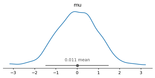
az.plot_rank(dt, var_names=["mu", "tau"], backend="matplotlib");
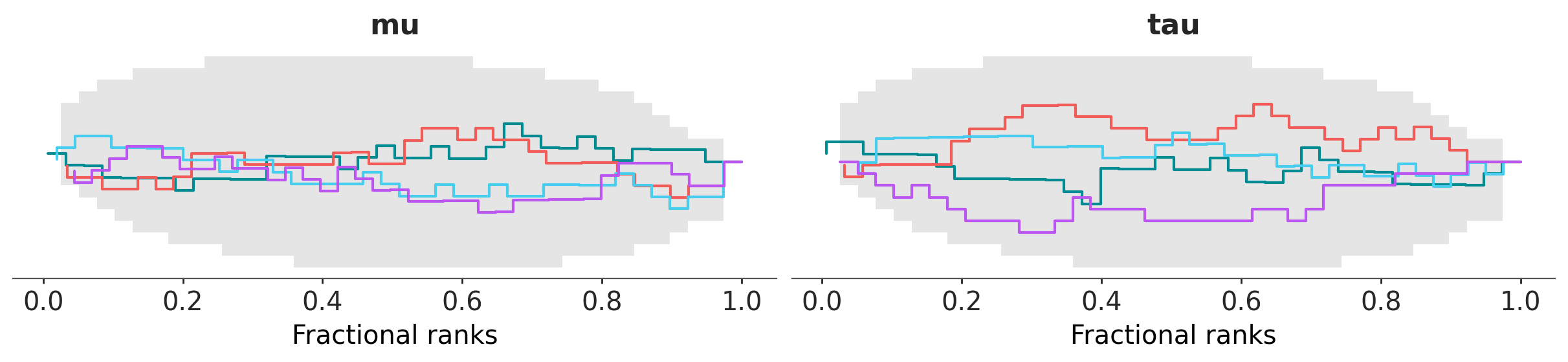
import plotly.io as pio
pio.renderers.default = "notebook"
pc = az.plot_rank(dt, var_names=["mu", "tau"], backend="plotly")
pc.show()
At the time of writing, there are three cross-backend themes defined by ArviZ:
arviz-variat, arviz-vibrant and arviz-cetrino.
Plotting function inventory#
The following functions have been renamed or restructured:
ArviZ <1 |
ArviZ >=1 |
|---|---|
plot_bpv |
plot_ppc_pit, plot_ppc_tstat |
plot_dist_comparison |
plot_prior_posterior |
plot_ecdf |
plot_dist, plot_ecdf_pit |
plot_ess |
plot_ess, plot_ess_evolution |
plot_forest |
plot_forest, plot_ridge |
plot_ppc |
plot_ppc_dist |
plot_posterior, plot_density |
plot_dist |
plot_trace |
plot_trace_dist, plot_trace_rank |
Others have had their code rewritten and their arguments updated to some extent, but kept the same name:
plot_autocorr
plot_bf
plot_compare
plot_energy
plot_khat
plot_lm
plot_loo_pit
plot_mcse
plot_pair
plot_parallel
plot_rank
The following functions have been added:
Some functions have been removed and we don’t plan to add them:
plot_dist (notice we have
plot_distbut it is a different function)plot_kde (this is now part of
plot_dist)plot_violin
And there are also functions we plan to add but aren’t available yet.
plot_elpd
plot_ppc_residuals
plot_ts
Note
For now, the documentation for arviz-plots defaults to latest which is built
from GitHub with each commit. If you see some of the functions in the last block already
on the example gallery you should be able to try them, but only if you install
the development version! See Installation
You can see all of them at the arviz-plots gallery.
What to expect from the new plotting functions#
There are two main differences with the plotting functions here in legacy ArviZ:
The way of forwarding arguments to the plotting backends.
The return type is now
PlotCollection, one of the key features ofarviz-plots. A quick overview in the context ofplot_xyzis given here but it later has a section of its own.
Other than that, some arguments have been renamed or gotten different defaults,
but nothing major. Note, however, that we have incorporated elements
from grammar of graphics into arviz-plots, now that we’ll cover the internals
of plot_xyz in passing we’ll use some terms from grammar of graphics.
If you have never heard about grammar of graphics we recommend you take
a look at Overview before continuing.
kwarg forwarding#
Most plot_xyz functions now have a visuals and a stats argument. These arguments
are dictionaries whose keys define where their values are forwarded too. The values
are also dictionaries representing keyword arguments that will be passed downstream
via **kwargs. This allows you to send arbitrary keyword arguments to all the different
visual elements or statistical computations that are part of a plot without
bloating the call signature with endless xyz_kwargs arguments like in legacy ArviZ.
These same arguments also allow indicating a visual element should not be added to the plot,
or providing pre computed statistical summaries for faster re-rendering of plots (at the time
of writing pre-computed inputs are only working in plot_forest but should be extended soon).
In addition, the call signature of new plotting functions is plot_xyz(..., **pc_kwargs),
with these pc_kwargs being forwarded to the initialization of PlotCollection.
This argument allows controlling the layout of the figure as well
as any aesthetic mappings that might be used by the plotting function.
For a complete notebook introduction on this see Introduction to batteries-included plots
New return type: PlotCollection#
All plot_xyz functions now return a “plotting manager class”. At the time of writing
this means either PlotCollection (vast majority of plots) or
PlotMatrix (for upcoming plot_pair for example).
These classes are the ones that handle faceting and
aesthetic mappings and allow the plot_xyz functions to
focus on the visuals and not on the plot layout or encodings.
See Using PlotCollection objects for more details on how to work with
existing PlotCollection instances.
Plotting manager classes#
As we have just mentioned, plot_xyz use these plotting manager classes and then return them
as their output. In addition, we hope users will use these classes directly to help them
write custom plotting functions more easily and with more flexibility.
By using these classes, users should be able to focus on writing smaller functions that take
care of a “unit of plotting”. You can then use their .map methods to apply these plotting
functions as many times as needed given the faceting and aesthetic mappings defined by the user.
Different layouts and different mappings will generally not require changes to these plotting
functions, only to the arguments that define aesthetic mappings and the faceting strategy.
Take a look at Create your own figure with PlotCollection if that sounds interesting!
Other arviz-plots features#
There are also helper functions to help compose or extend existing plotting functions.
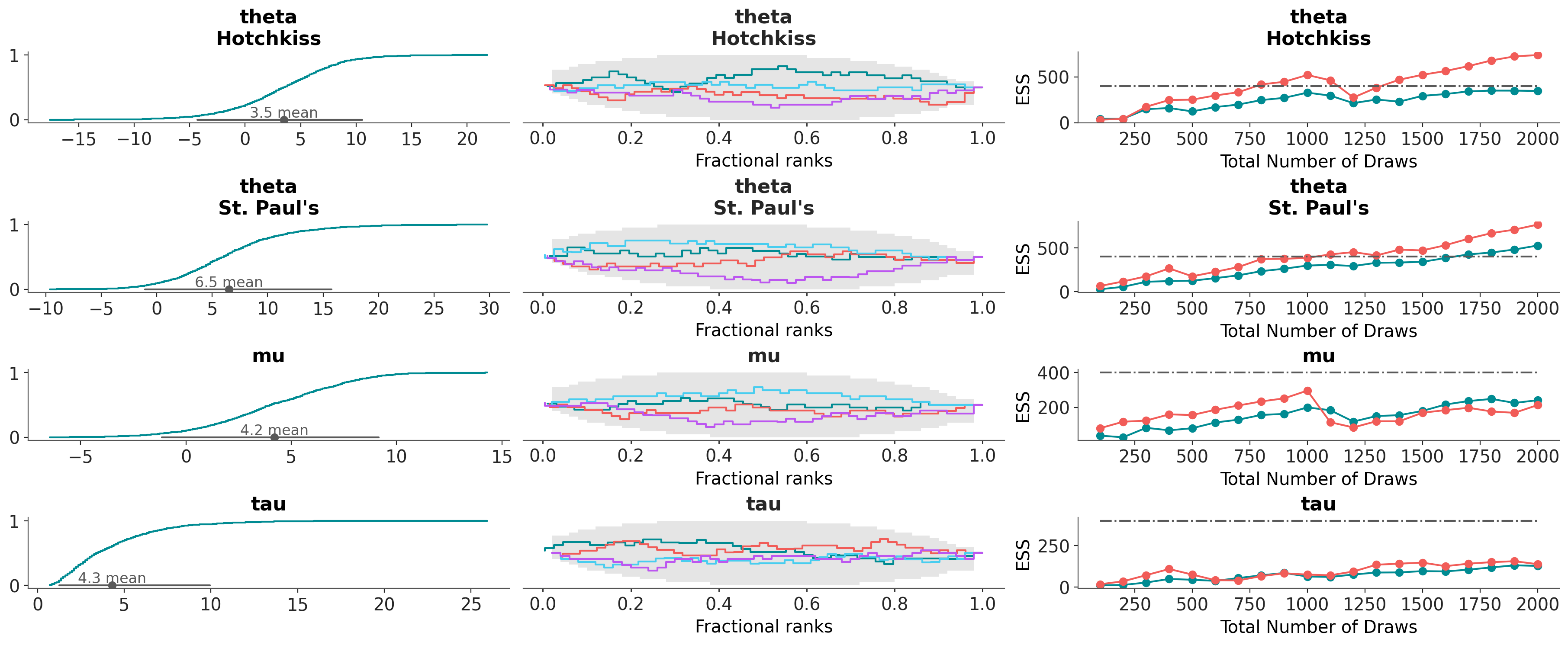
For example, we can create a new plot, with a similar layout to that of plot_trace_dist
or plot_rank_dist but custom diagnostics in each column: distribution, rank and ess evolution:
az.combine_plots(
dt,
[
(az.plot_dist, {"kind": "ecdf"}),
(az.plot_rank, {}),
(az.plot_ess_evolution, {}),
],
var_names=["theta", "mu", "tau"],
coords={"school": ["Hotchkiss", "St. Paul's"]},
);
Other nice features#
Citation helper#
We have also added a helper to cite ArviZ in your publications and also the methods implemented in it.
You can get the citation in BibTeX format through citation():
Extended documentation#
One recurring feedback we have received is that the documentation was OK for people very familiar with Bayesian statistics and probabilistic programming, but not so much for newcomers. Thus, we have added more introductory material and examples to the documentation, including a separated resource that show how to use ArviZ “in-context”, see EABM. And we attempted to make the documentation easier to navigate and understand for everyone.